The recommended way to specify custom priors is demonstrated in the code below. It puts an ex-Gaussian prior on alpha (ex-Gaussian is often used to model skewed distributions including RTs) and puts a Normal prior on slopes. Strategy can be extended to put any custom prior on any of the PF's parameters. No idea whether specific choices (e.g., for the parameter values of the ex-Gaussian) I made in this example would be appropriate for any specific situation.
The code below produces this image of the prior (I rotated view though for clarity):
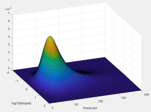
Code: Select all
priorAlphaRange = linspace(0,200,201);
priorBetaRange = linspace(-2,2,101);    %log10 transformed values as usual
priorGammaRange = 0.5;
priorLambdaRange = .03;

%set up PM structure (with uniform prior for now):
PM = PAL_AMPM_setupPM('priorAlphaRange',priorAlphaRange,'priorBetaRange',priorBetaRange,'priorGammaRange',priorGammaRange,'priorLambdaRange',priorLambdaRange,'PF',@PAL_CumulativeNormal);

%PM.priorAlphas now has the same dimensions as the full prior/posterior
%distribution (i.e., 201 x 101) and contains, for each position in the array,
% the value of the threshold parameter.

%PM.priorBetas now has the same dimensions as the full prior/posterior
%distribution (i.e., 201 x 101) and contains, for each position in the array,
%the value of the slope parameter.

%similar for PM.priorGammas and PM.priorLambdas, but these will be constant
%in this example.

%Defining non-uniform prior across multi-dimensional parameter space is now
%easy.
%The following puts an exGaussian density on threshold and a Gaussian
%density on slopes:
prior = PAL_pdfExGaussian(PM.priorAlphas,30,10,30).*PAL_pdfNormal(PM.priorBetas,0,.5);

%normalize:
prior = prior./sum(sum(prior));

%update PM structure with new prior (other previously defined settings are
%not affected by this):
PM = PAL_AMPM_setupPM(PM,'prior',prior);

%visualise prior
surf(priorBetaRange, priorAlphaRange,squeeze(PM.pdf))
xlabel('log10(slopes)');
ylabel('threshold');

